The Jacobian vs. the Hessian vs. the Gradient

What are the differences between the Jacobian, the Hessian and the Gradient? All three have ties to multivariable calculus, let's dive in and take a look!

Keywords: multivariable calculus, artificial intelligence, optimization, physics

By Carmen Cincotti

August 15, 2022

The Gradient
- A scalar-valued function
- How to calculate the Gradient
The Hessian
- The Hessian determinant
The Jacobian
- The determinant of the Jacobian matrix
Resources

When studying multivariable calculus, we often come across the use of matrices to represent different concepts. We often come across the Jacobian, the Hessian and the gradient.

Jacobian vs Hessian

These concepts are close to each other, by virtue of being matrices having to do with derivatives of functions, However, each matrix has its own derivation, and signification.

What is the difference between the Jacobian, the Hessian and the gradient 🤔? We will discover it together in this article. During this mathematical journey, we will also study the concepts of the difference between vector-valued functions and scalar-valued functions.

The Gradient

We start with the gradient which we already talked about a few weeks ago. The gradient is a vector composed of the partial derivatives of a scalar-valued function, $f$ :

\nabla{f}(x, y, z) = \begin{bmatrix} \frac{\partial f}{\partial x} \\[6pt] \frac{\partial f}{\partial y} \\[6pt] \frac{\partial f}{\partial z} \\ \end{bmatrix}

where $\nabla$ is called nabla. It is sometimes called “del”. It denotes the vector differential operator.

Recall that the gradient measures the direction and the fastest rate of increase of a function $f$ at a given point.

Let’s imagine that we are at the foot of a mountain, and we wanted to climb it as quickly as possible. We see that the right track is to climb it in the direction of the arrow:

Person climbing a mountain

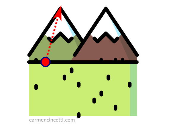
This arrow represents the gradient because it is the fastest ascent up the mountain.

A scalar-valued function

A scalar-valued function is a function (multi-variable / of dimension $n$ ) that returns a scalar value:

f: \mathbb{R}^n \rightarrow \mathbb{R}

For example, if we evaluate $f(x,y) = x + y$ at the point (2,1), we get the scalar, 3:

f(2,1) = 2 + 1 = 3\\[6pt]

How to calculate the Gradient

Let’s take an example. I have a function defined as $f(x,y) = 5x^2 + 3xy + 3y^3$ . First, we need to find the partial derivatives with respect to the variables $x$ and $y$ as follows:

\frac{\partial f}{\partial x} = 10x + 3y \\[6pt] \frac{\partial f}{\partial y} = 3x + 9y^2 \\[6pt]

This gives us a gradient:

\nabla{f} = \begin{bmatrix} 10x + 3y \\[6pt] 3x + 9y^2 \\ \end{bmatrix}

The Hessian

If we follow the explanation of the gradient, the Hessian will also be easy to understand. It is the derivative of the gradient of a scalar-valued function $f: \mathbb{R}^n \rightarrow \mathbb{R}$ . For instance :

\mathbf{H}f(x, y) = \nabla{}^2f(x, y) = \begin{bmatrix} f_{xx} & f_{xy} \\[6pt] f_{yx} & f_{yy} \\[6pt] \end{bmatrix}

Using again the function $f(x,y) = 5x^2 + 3xy + 3y^3$ , we will see a Hessian matrix as follows:

\mathbf{H}f(x, y) = \nabla{}^2f(x, y) = \begin{bmatrix} 10 & 3 \\[6pt] 3 & 18y \\[6pt] \end{bmatrix}

Some applications of the Hessian matrix are the following:

Quadratic approximations of a multivariable function. This is a closer approximation to the function than the local linear approximation we already discussed several weeks ago.
The partial second derivative test - it is used to find saddle points, the maxima and the minima of a function.

The Hessian determinant

The Hessian determinant plays a role in finding the local maxima/minima of a multivariable function. We will see what a determinant is in a later article. For now, I’ll just explain how to calculate it. I present to you once again the Hessian matrix that we have already calculated in the last part:

\mathbf{H}f(x, y) = \nabla{}^2f(x, y) = \begin{bmatrix} 10 & 3 \\[6pt] 3 & 18y \\[6pt] \end{bmatrix}

In order to find the determinant, we need to follow the framework below:

\det\begin{pmatrix}\begin{bmatrix} a & b \\[6pt] c & d \\[6pt] \end{bmatrix}\end{pmatrix} = ad-bc

Therefore,

\det\begin{pmatrix}\begin{bmatrix} 10 & 3 \\[6pt] 3 & 18y \\[6pt] \end{bmatrix}\end{pmatrix} = 180y - 9

The Jacobian

The Jacobian is a matrix that holds all first-order partial derivatives of a vector-valued function:

f: \mathbb{R}^n \rightarrow \mathbb{R}^n

The Jacobian form of a vector-valued function $h(f(x,y), g(x, y))$ is therefore the following:

\mathbf{J}h(f(x,y), g(x,y)) = \begin{bmatrix} f_x & f_y \\[6pt] g_x & g_y \\[6pt] \end{bmatrix}

For example - if we have a vector-valued function like:

f(x,y): \begin{bmatrix} sin(x) + y \\[6pt] x + cos(y) \end{bmatrix}

The Jacobian matrix will be :

J(f) = \begin{bmatrix} cos(x) & 1 \\[6pt] 1 & -sin(y) \end{bmatrix}

By using the Jacobian, we can locally linearize a vector valued function at a specific point.

Linear functions are simple enough that we can understand them well (using linear algebra), and often understanding the local linear approximation of $f(x,y) allows us to draw conclusions about$ f $$ itself.

To learn more about the calculation, here is a video that helped me a lot:

The determinant of the Jacobian matrix

We can use Jacobian matrix of a vector valued transformation to find its determinant. To do this with a transformation of $f: \mathbb{R}^3 \rightarrow \mathbb{R}^3$ , we use the framework:

\det\begin{pmatrix}{\begin{bmatrix} a_1 & a_2 & a_3 \\[6pt] b_1 & b_2 & b_3 \\[6pt] c_1 & c_2 & c_3 \\[6pt] \end{bmatrix}}\end{pmatrix} = a_1 \det\begin{pmatrix}\begin{bmatrix} b_2 & b_3 \\[6pt] c_2 & c_3 \\[6pt] \end{bmatrix}\end{pmatrix} - a_2 \det\begin{pmatrix}\begin{bmatrix} b_1 & b_3 \\[6pt] c_1 & c_3 \\[6pt] \end{bmatrix}\end{pmatrix} + a_3 \det\begin{pmatrix}\begin{bmatrix} b_1 & b_2 \\[6pt] c_1 & c_2 \\[6pt] \end{bmatrix}\end{pmatrix}

Consider this example using this Jacobian matrix:

J(f)=\begin{bmatrix} 2xy & x^2 & 0 \\[6pt] 0 & -1 & 1 \\[6pt] 1 & 0 & 1 \end{bmatrix}

We can calculate the determinant as follows:

\det\begin{pmatrix}\begin{bmatrix} 2xy & x^2 & 0 \\[6pt] 0 & -1 & 1 \\[6pt] 1 & 0 & 1 \end{bmatrix}\end{pmatrix} = 2xy \det\begin{pmatrix}\begin{bmatrix} -1 & 1 \\[6pt] 0 & 1 \\[6pt] \end{bmatrix}\end{pmatrix} - x^2 \det\begin{pmatrix}\begin{bmatrix} 0 & 1 \\[6pt] 1 & 1 \\[6pt] \end{bmatrix}\end{pmatrix} + 0 \det\begin{pmatrix}\begin{bmatrix} 0 & -1 \\[6pt] 1 & 0 \\[6pt] \end{bmatrix}\end{pmatrix}

= 2xy(-1(1) - (1(0))) - x^2(0(1) - 1(1)) + 0(0(0) - (-1(1)))\\[6pt] = 2xy(-1) - x^2(-1) + 0 \\[6pt] = -2xy + x^2

What does the determinant mean? 🤔 The function $-2xy+x^2$ gives us the amplitude in which space contracts or expands during a transformation around a point $(x, y, z)$ .

For example, if we evaluate it at the point $(1, 0, 2)$ , we will see:

= -2(1)(0) + 1^2 \\[6pt] = 0 + 1 \\[6pt] = 1

Which tells us that the space does not change around this point! However, around the point $(3, 1, 0)$ , we see another story:

= -2(3)(1) + 3^2 \\[6pt] = -6 + 9 \\[6pt] = 3

I recommend this resource in order to visualize the transformations and the determinant for each one!

Carmen's Graphics Blog