I just keep hitting walls when it comes to my fabric simulation! While reading this article on position based dynamics, I came across the concept of local linearization of nonlinear functions. The author mentioned that:

The problem, as always, is that this concept was unknown to me. 🤦‍♂️

We have already talked about nonlinear functions when discussing the topic of constrained functions in this article. We will continue this discussion in the context of simplifying these functions by linearizing them.

Why should I care? 🙋 Solving non-linear functions can be an expensive task, depending on its complexity. Through linearization, it is possible to partition linear parts of a non-linear function to solve them with much simpler linear equations. This is to solve them more easily and at a lower cost of resources!

Linearization with tangential planes

To start, let’s quickly define the difference between a linear function and a nonlinear function:

• Linear - a function that makes a straight line when drawn. For example, let’s take a look at this graph together for the function $y = 2x + 1$:

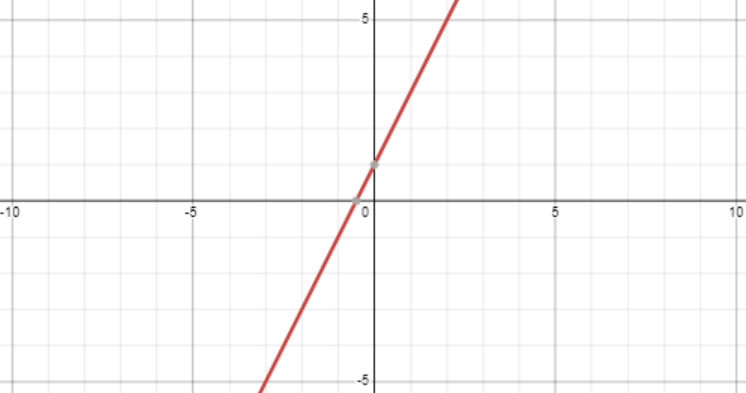
Note that these functions take the form:

For example:

You may also notice that the partial derivatives are constant. For example — a function like $g(x,y) = ax + by + c$ will have constant partial derivatives:

• Nonlinear - these are functions that do not take on straight lines when drawn. Here is the non-linear function $y = x^2 - 1$ :

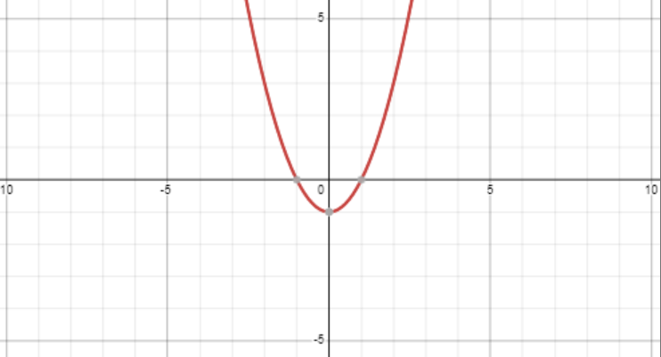
Unlike linear functions, the partial derivatives of a non-linear function are not entirely constant. Here are the partial derivatives of a function $g(x,y) = x^2 + y^2 + 1$:

Linearization of a nonlinear function can be summarized by saying that we would like to find a plane tangential to a point on a graph of a nonlinear function. This plane function serves as the linear function at that given point.

To clarify, here is the graph for the nonlinear function $f(x,y) = x^2+ y^2$ (blue) and a tangent plane represented by the function $g(x,y) = 2(x-1) + 2(y-1) + 2$ (purple) :

At the point $(1, 1)$, the two functions intersect. We can say that at the point $(1,1)$ the function is linearized as $g(x,y)$.

However, this linearization will get worse the further we get from the point $(1,1)$. This is why we should say that the function $f(x, y)$ is linearized locally at the point $(1, 1)$.

Since we are now more familiar the concept of linearization, we can examine it more closely. Remember that our goal is to understand this equation:

The tangent plane

In the last section, I used a function $g(x,y)$ to describe a plane. However, it seems a bit too magical. 🪄

How ​​to find the equation of a plane? To start, here is the equation of a plane in its entirety:

By using a normal vector and two points that lie on the plane, it is possible to find its equation.

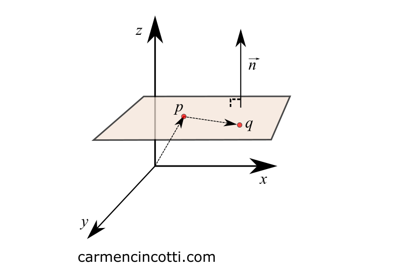
where $\vec{n} = (a,b,c)$ and $\vec{pq} = (x_q - x_p, y_q - y_p, z_q - z_p)$. $\vec{pq}$ lies entirely on the plane.

We know that the dot product between two perpendicular vectors is equal to 0. Which leaves us with the following form $\vec{n} \cdot \vec{pq} = 0$.

Finally, I will rewrite this equation in a form where the vector $\mathbf{x_0}$ is the intersection position of the plane and a nonlinear function:

Keep this equation in mind because we will see it in the next part!

Local linearization

Since we now know the equation of a plane - we can add to this knowledge. Suppose we want to approximate the earlier function $f(x,y) = x^2+ y^2$ by finding its local linear approximation.

To do this, we want to find a function of a plane that is tangent to the function at point $(x,y,z)$.

The inputs to the function $f(x,y)$ give us the value $z$. So we can say that the plane and the function $f(x,y)$ intersect at the point $(x, y, f(x,y))$.

Then, we can rewrite the equation of a plane $a(x - x_0) + b(y - y_0) + c(z - z_0) = 0$ to get rid of the variable $c$ and to separate $z$:

How shall we continue? 🤔

An important characteristic of a tangential curve

Well, the most important thing to remember when talking about tangential curves is that a curve and its tangential counterpart must have the same slope at the point of intersection!

Otherwise, they cannot be tangential. Look at these two 2D graphs:

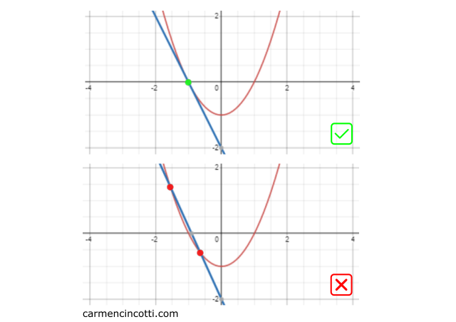
• The top graph shows two lines that barely intersect at a single point - $(-1.0)$, which means that the blue curve is tangent to the red curve. ✅

• The bottom graph has two intersections which means that the blue line is not tangential to the red curve. ⛔

You may be wondering:

How can we find the slope of $f(x,y)$ ? 🤔

The slope is the gradient $\nabla f(x,y)$! Recall that the gradient consists of the partial derivatives of a multivariable function.

Using the partial derivatives of $f(x,y)$ - $f_x$ and $f_y$ - we can assume that:

Finally, we rewrite this equation with the knowledge that the two points intersect at point $(x, y, f(x,y))$ and by setting $L_f(x,y) = f(x,y ) = z$ to be clear that the function $L_f(x,y)$ is the local linear approximation of $f(x,y)$ :

Function rewrite

Recall the linear function that we used is as follows:

We can rewrite our function $L_f(x,y)$ in this form using $\mathbf{x} = (x, y)$ and $\mathbf{x}_0 = (x_0, y_0 )$:

…which is the same form of the constrained function from the introduction, but where $\mathbf{x}_0 = x$ and $\mathbf{x} = x+\Delta x$ :

Resources

• Linear and Non-Linear Functions
• Equations of Planes - Paul’s Online Notes
• Scalar Equation of a Plane - J. Garvin
• Tangent Planes and Linear Approximations - Paul’s Online Notes
• What are the benefits of linearization? - Stack Exchange